Survival
生存分析:研究因素与生存结局(阳性结局)在时间跨度上的关联
| 数据组成 | |
|---|---|
| 分组信息 | e.g.A型血,B型血,O型血,AB型血 |
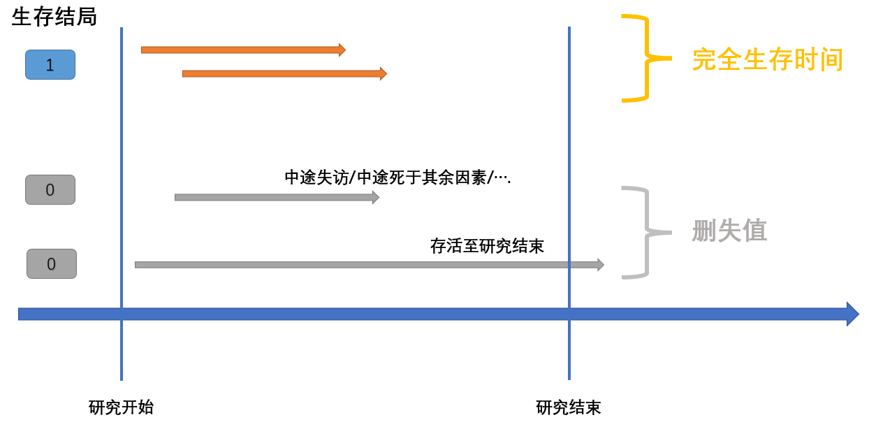
| 生存结局 | 研究者设定某种阳性事件(e.g.死亡)。研究进行的时间跨度中,若事件发生则结局为1,若未发生则结局为0 |
| 生存时间 | 从随访至阳性事件所经历的时间。可分为完全生存时间与非完全生存时间(又称截尾值/删失值,censord value) |
| 分析手段 | |
|---|---|
| 描述生存过程 | K-M曲线 |
| 生存/风险曲线是否有差异 | LogRank(Mantel-Haenszel): 各时间点权重一样,对远期差异敏感 Gehan Wilcoxon(Breslow): 以各时间点的观察例数为权重,对早期差异敏感 Tarone-Ware: 以各时间点的观察例数的平方根为权重 详细link,根据事件时间分布、删失分布、曲线是否交叉 来决定方式与看待结果 |
| 寻找风险因素 | Cox 回归模型 |
| 术语 | ||
|---|---|---|
| 生存函数 | $$S(t)=P(T>t)$$ | 个体的生存时间大于t的概率 |
| (ti时刻生存概率) | $$S(t_i)=S(t_{i-1})(1-\frac{d_i}{n_i})=exp[-\int_{0}^{t}h(u)du]$$ | d_i:在ti死亡的数目 n_i: ti之前存活且非数据删失的数目 |
| 风险函数 $\lambda$ | $$h(t)=\lim\limits_{\Delta t\rightarrow0}\frac{P(t\leq T<t |T\geq t)}{\Delta t}=-\frac{dS(t)/dt}{S(t)}$$ | 个体生存到t时刻,单位时间内事件发生的rate |
| Cox 模型 | $$h(t)=h_0(t)*\exp(b_1x_1+b_2x_2+...+b_px_p)$$ | $b>0增加h(t),b=0于h(t)无影响,b<0减小h(t)$ |
| Hazard Ratio | $$\frac{h_0(t)*\exp(b_1(x_1+1)+b_2x_2+...+b_px_p)}{h(t)}$$ | 若x_1增加一个单位,增加前后的风险对比,详见 |
R示例
Data
lung数据集,数据详情及下载见链接。
setwd('C:\\Users\\12990\\Desktop\\s')
library("survival")
library("survminer")
lung <-read.csv("dataset-68740.csv",head=T,check.names=F)
Fit
Surv()创建一个生存对象,随后survfit()创建一个分析图
Surv(time,event)

## time:  time
## event: 阳性事件发生的状态
如下写法数值一致
> survfit(Surv(lung$time,lung$status==2) ~ lung$sex)
Call: survfit(formula = Surv(lung$time, lung$status == 2) ~ lung$sex)

             n events median 0.95LCL 0.95UCL
lung$sex=1 138    112    270     212     310
lung$sex=2  90     53    426     348     550

> survfit(Surv(time,status==2) ~ sex , data = lung)
Call: survfit(formula = Surv(time, status == 2) ~ sex, data = lung)

        n events median 0.95LCL 0.95UCL
sex=1 138    112    270     212     310
sex=2  90     53    426     348     550


n: 样本数
events: 阳性事件发生数
median: 中位生存率对应的生存时间
0.95LCL: 置信区间下限
0.95UCL: 置信区间上限
K-M
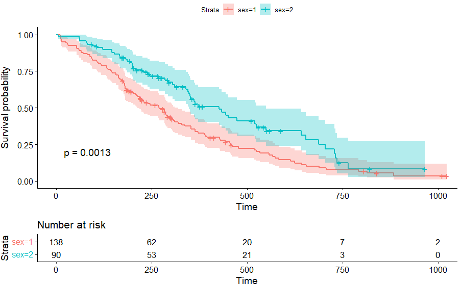
KM_sex <- survfit(Surv(time,status==2) ~ sex , data = lung)
p1 = ggsurvplot(KM_sex,
                pval = TRUE,
                ggtheme = theme_bw(),
                conf.int = TRUE,
                risk.table = TRUE,
                fun="event")


## "event" plots cumulative events (f(y) = 1-y),
## "cumhaz" plots the cumulative hazard function (f(y) = -log(y)),
## "pct" for survival probability in percentage.
## arrange_ggsurvplots(list(p1,p2,p3))
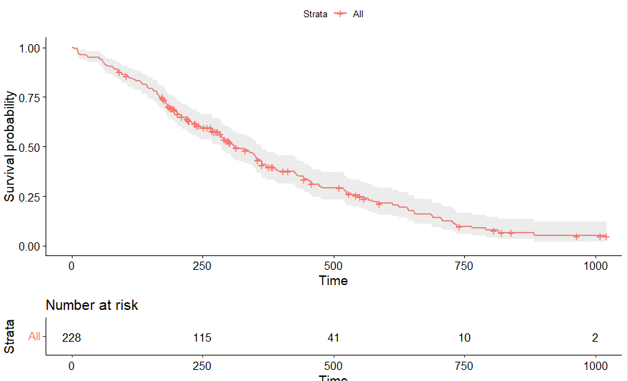
KM_all <- survfit(Surv(time,status==2) ~ 1 , data = lung)
ggsurvplot(KM_all,pval = TRUE, conf.int = TRUE,risk.table = TRUE)

#plot(KM_all,conf.int=T,col=c("red"),xlab="Days",ylab = "Survival probability")
#legend(0,0.5,legend=c("All"),lty=1,col=c("red"))
> summary(KM_all)
Call: survfit(formula = Surv(time, status == 2) ~ 1, data = lung)

 time n.risk n.event survival std.err lower 95% CI upper 95% CI
    5    228       1   0.9956 0.00438       0.9871        1.000
   11    227       3   0.9825 0.00869       0.9656        1.000
   12    224       1   0.9781 0.00970       0.9592        0.997
   13    223       2   0.9693 0.01142       0.9472        0.992
   15    221       1   0.9649 0.01219       0.9413        0.989
   26    220       1   0.9605 0.01290       0.9356        0.986
......
log-rank test
- 参考: With default rho = 0 this is the log-rank or Mantel-Haenszel test, and with rho = 1 it is equivalent to the Peto & Peto modification of the Gehan-Wilcoxon test
surv_diff <- survdiff(Surv(time, status) ~ sex, data = lung, rho = 0)
p.val = surv_diff$pvalue
> surv_diff
Call:
survdiff(formula = Surv(time, status) ~ sex, data = lung)

        N Observed Expected (O-E)^2/E (O-E)^2/V
sex=1 138      112     91.6      4.55      10.3
sex=2  90       53     73.4      5.68      10.3

 Chisq= 10.3  on 1 degrees of freedom, p= 0.001
COX
- 基于风险比模型,评估不同变量对生存率的影响;Cox模型和log-rank test都要求风险等比例(PH假定,Assumptions,pre-test),若否,可尝试RMST、分层、时依协变量、等方法
- 在进行多元回归前,如果因子太多,可以使用survdiff分组检验先选出显著的因子。
- 除了Cox模型外,还要一些拟合其它分布的模型,例如指数、Weibull、Gompertz分布
单因素
单因素拟合Cox比例风险回归模型。风险比率exp(coef)=0.5880,说明女性(2)死亡风险是男性(1)的0.5880倍。
cox_sex <- coxph(Surv(time,status==2) ~ sex , data = lung)

> cox_sex
Call:
coxph(formula = Surv(time, status == 2) ~ sex, data = lung)

       coef exp(coef) se(coef)      z       p
sex -0.5310    0.5880   0.1672 -3.176 0.00149

Likelihood ratio test=10.63  on 1 df, p=0.001111
n= 228, number of events= 165
多因素
cox_2 <- coxph(Surv(time,status==2) ~ sex +age, data = lung)
> summary(cox_2)
Call:
coxph(formula = Surv(time, status == 2) ~ sex + age, data = lung)

  n= 228, number of events= 165

         coef exp(coef)  se(coef)      z Pr(>|z|)
sex -0.513219  0.598566  0.167458 -3.065  0.00218 **
age  0.017045  1.017191  0.009223  1.848  0.06459 .
---
Signif. codes:  0 ‘***’ 0.001 ‘**’ 0.01 ‘*’ 0.05 ‘.’ 0.1 ‘ ’ 1

    exp(coef) exp(-coef) lower .95 upper .95
sex    0.5986     1.6707    0.4311    0.8311
age    1.0172     0.9831    0.9990    1.0357

Concordance= 0.603  (se = 0.025 )
Likelihood ratio test= 14.12  on 2 df,   p=9e-04
Wald test            = 13.47  on 2 df,   p=0.001
Score (logrank) test = 13.72  on 2 df,   p=0.001
分层
加strata()按age分层计算,减少age造成的扰动
Call:
coxph(formula = Surv(time, status == 2) ~ sex + strata(age),
    data = lung)

       coef exp(coef) se(coef)      z       p
sex -0.6447    0.5248   0.2120 -3.041 0.00236

Likelihood ratio test=9.79  on 1 df, p=0.001756
n= 228, number of events= 165
Hazard Ratio
> summary(cox_sex)$coef[2]
[1] 0.5880028
PH假定
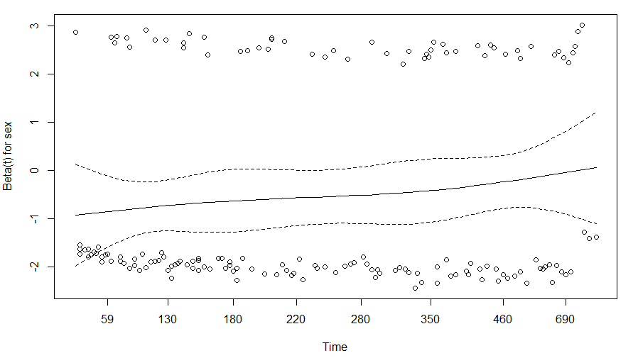
H0假设:风险比不会随时间而变化。p>0.05,不能拒绝H0。
如果风险比伴随时间变化(p<=0.05),方程中可加入类似'var*time'的变换。
## 图形法检验PH假定
plot(cox.zph(cox_2,transform=rank),var='sex')

> cox.zph(cox_2,transform=rank)
       chisq df    p
sex    2.378  1 0.12
age    0.137  1 0.71
GLOBAL 2.475  2 0.29
Predict
使用COX模型预测生存时间(待确认)
fit <- survreg(Surv(time, status) ~ ph.ecog, data=lung)
pred <- <- predict(fit, newdata=data.frame(ph.ecog=2), type='quantile',p=pct, se=TRUE)
模型检验: C-index
预测模型的评价指标一般需要考虑:区分能力(ROC),一致性(goodness-of-fit/C-index),其它例如回归模型的 MSE、R2等。对 COX 回归模型的评价一般使用 C-index,上述代码的结果中已经提供 summary(cox_2)$concordance (不确定是那种C-index?待确认)
此外还可以使用 Hmisc 包进行计算 Harrell’s C
library(survival)
library(Hmisc)
fit <- survdiff(Surv(time, status) ~ sex, data = lung, rho = 0)
pred <- predict(fit)
HarrellC <- 1-rcorr.cens(pred,Surv(time,status))
C-index 的计算过程是:将所有样本两两组合,预测其生存时间;若一对样本的label显示S1的生存时间长于S2,预测值也符合这一关系,则这一对样本归为“Concordance”;最终,C-index = Concordance_pairs/all_pairs
RR,OR,HR
| -- | 发生 Risk=1 | 未发生 Risk=0 |
|---|---|---|
| 暴露组 Exposure=1 | a | b |
| 非暴露组 Exposure=0 | c | d |
- Relative Risk: 暴露组Risk率/非暴露组Risk率   (发病/死亡率)
RR = P(Risk=1|Exposure=1) / P(Risk=1|Exposure=0)
   = [a/(a+b)] / [c/(c+d)]

- Odd Ratio: Risk组(暴露_非暴露)比值/非Risk组(暴露_非暴露)比值
OR = [a/c] / [b/d]

- Hazard Ratio: 考虑了时间因素的RR
HR 见 上文
可以将log(OR)作为GWAS分析的表型,寻找可能的致病位点
参考
Survival-R: https://zhuanlan.zhihu.com/p/130316068
Survival: http://thisis.yorven.site/blog/index.php/2020/04/06/survival-analysis/
ggsurvplot:https://zhuanlan.zhihu.com/p/113676828
Survival: https://zhuanlan.zhihu.com/p/497968260
KM: https://zhuanlan.zhihu.com/p/391474891
检验:http://www.lcgdbzz.org/custom/news/id/9442
RR,OR,HR:https://blog.csdn.net/weixin_41858481/article/details/95773773
C-index 5种方法: https://blog.csdn.net/weixin_41368414/article/details/123660946
C-index: https://blog.csdn.net/fjsd155/article/details/84669331